Noise in Creative Coding
Noise is an indispensable tool for creative coding. We use it to generate all kinds of organic effects like clouds, landscapes and contours. Or to move and distort objects with a more lifelike behaviour.
On the surface, noise appears to be simple to use but, there are so many layers to it. This post takes a deep dive into what noise is, its variants, how to use it on the web and its applications. And lot’s of examples. So many examples!
What is noise?
Imagine you want to move an object around the screen. Animators will use keyframes and tweens to describe the exact motion. Generative artists instead rely on algorithms.
So what, something like math.random()?
Not exactly. Randomness is just too unnatural. Look at that pink ball, bouncing all over the place. It’s nauseating 🥴
What we need is a smoother, more organic randomness. That is what the noise function generates (the yellow ball). Much more aesthetically pleasing!
This idea of organic randomness appears again and again in creative coding. For example, when generating textures, moving objects or distorting them. We often reach for the noise function.
Generating noise on the web
There are two flavours of noise—Perlin and Simplex.
Ken Perlin developed the first while working on Tron in the early 1980s and won an Oscar 🏆 for those special effects. He then improved on it with Simplex noise and made it a bit faster. I’ll focus on the latter and use the simplex-noise library for my examples.
The noise function takes in a couple of inputs (which drive the output) and returns a value between -1 and 1. The output is a mix of Math.sin() and Math.random(). A random wave is how I would describe it.
import SimplexNoise from 'simplex-noise';

const simplex = new SimplexNoise();
const y = simplex.noise2D(x * frequency, 0) * amplitude;
The underlying mechanics are similar to how waves work. You can control how quickly or how much it oscillates by adjusting frequency and amplitude.
Umm, noise… 2D, what’s happening here?
Noise Dimensions
The noise algorithm can be implemented for multiple dimensions. Think of these as the number of inputs into the noise generator—two for 2D, three for 3D and so on.
Which dimension you pick depends on what variables you want to drive the generator with. Let’s look at a few examples.
💡 Starting here, each example is embedded in a source card. With links to the actual source code and, in some cases, variables you can tweak.
Noise 1D — Wave Motion
Technically there is no noise1D. You can get 1D noise by passing in zero as the second argument to simplex.noise2D. Let’s say you want to move a ball with an organic-looking oscillating motion. Increment its x coordinate and use it to generate the y value.
x += 0.1;
y = simplex.noise2D(x * frequency, 0) * amplitude;Noise2D — Terrain Generator
We can turn a flat 2D plane into hilly terrain by moving its vertices in the z-direction. Use the x and y coordinates to generate the z location.
And just like that, we have a terrain generator 🏔️
z = simplex.noise2D(x * frequency, y * frequency) * amplitude;Noise3D — Vertex Displacement
You’ve probably seen these distorted spheres in the wild. They are created by displacing the vertices of a sphere. Use the vertex coordinate (x, y, z) to generate the distortion amount. Then displace the vertex by it radially.
const distortion =
  simplex.noise3D(x * frequency, y * frequency, z * frequency) * amplitude;

newPosition = position.normalize().multiplyScalar(distortion);Noise4D — Animated Distortion
We can animate the distorted sphere by using 4D noise. The inputs will be the vertex coordinate (x, y, z) and time. This technique is used to create fireballs, amongst other things.
const distortion =
  simplex.noise4D(
    x * frequency,
    y * frequency,
    z * frequency,
    time * frequency
  ) * amplitude;

newPosition = position.normalize().multiplyScalar(distortion);Notice our use of amplitude in the above examples. It’s a handy way to scale the noise output to your application. You could also use interpolation to map the noise output to a specified range of your choice.
Now that we have the basics down let’s look at a few more applications of noise.
Textures
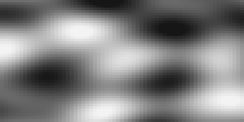
The noise output for a 2D grid, with (x,y) coordinates, looks something like this:

Generated using:
for (let y = 0; y < gridSize[1]; y++) {
  for (let x = 0; x < gridSize[0]; x++) {
    const n = simplex.noise2D(
      x / (gridSize[0] * 0.75),
      y / (gridSize[1] * 0.75)
    );
  }
}
This is going to be our starting point.
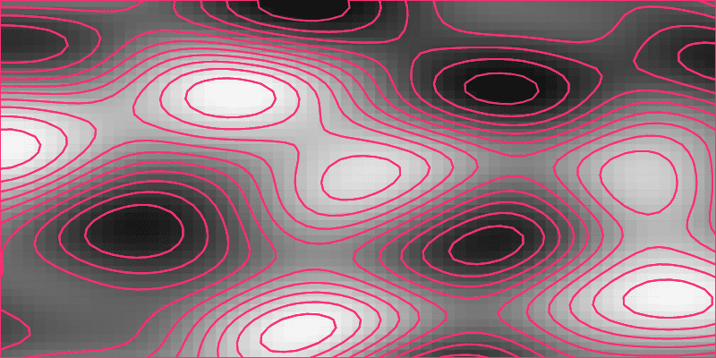
We can use the Marching Squares algorithm to turn that 2D noise data into contours. Using Canavas, SVG, WebGL or whatever else you prefer. I recently used this technique with SVG to create generative profile cards. For a full tutorial on that, check out creating a generative image service 📸

The cool thing about noise is that you can go up one dimension, layer in time and animate your image.
simplex.noise3D(x / (gridSize[0] * 0.75), y / (gridSize[1] * 0.75), time);Fields
Honestly, this 2D grid of noise data is super utilitarian. It’s my go-to for all kinds of stuff. One of which is noise fields—a particular favourite of mine.
Let’s go back to that initial grayscale output. Map that to a more interesting colour scale, and you get plasma 🤩
Or, start with a grid of rectangles. Then turn it into a vector field by using noise to control the colour and angle of rotation.
Noisy Particles
Vector fields are cool, but flow fields are an even more exciting visualization. Here’s a plot I made last year.
Notice the path that the pen traces. Each one of those strokes is generated by dropping a particle onto the vector field. And then tracing its path. 💫
Alright, let’s break down this process.
Creating a Flow Field
Step 1, create a vector field. Same as before. But this time, we’re not going to animate the vector field.
Step 2, drop a bunch of particles onto the canvas. Their direction of movement is based on the underlying vector field. Take a step forward, get the new direction and repeat.
function moveParticle(particle) {
  // Calculate direction from noise
  const angle =
    simplex.noise2D(particle.x * FREQUENCY, particle.y * FREQUENCY) * AMPLITUDE;

  // Update the velocity of the particle
  // based on the direction
  particle.vx += Math.cos(angle) * STEP;
  particle.vy += Math.sin(angle) * STEP;

  // Move the particle
  particle.x += particle.vx;
  particle.y += particle.vy;

  // Use damping to slow down the particle (think friction)
  particle.vx *= DAMPING;
  particle.vy *= DAMPING;

  particle.line.push([particle.x, particle.y]);
}
Step 3, track the location of the particle to trace its path.
Add in more particles and colour, and we get our flow field.
Particle systems
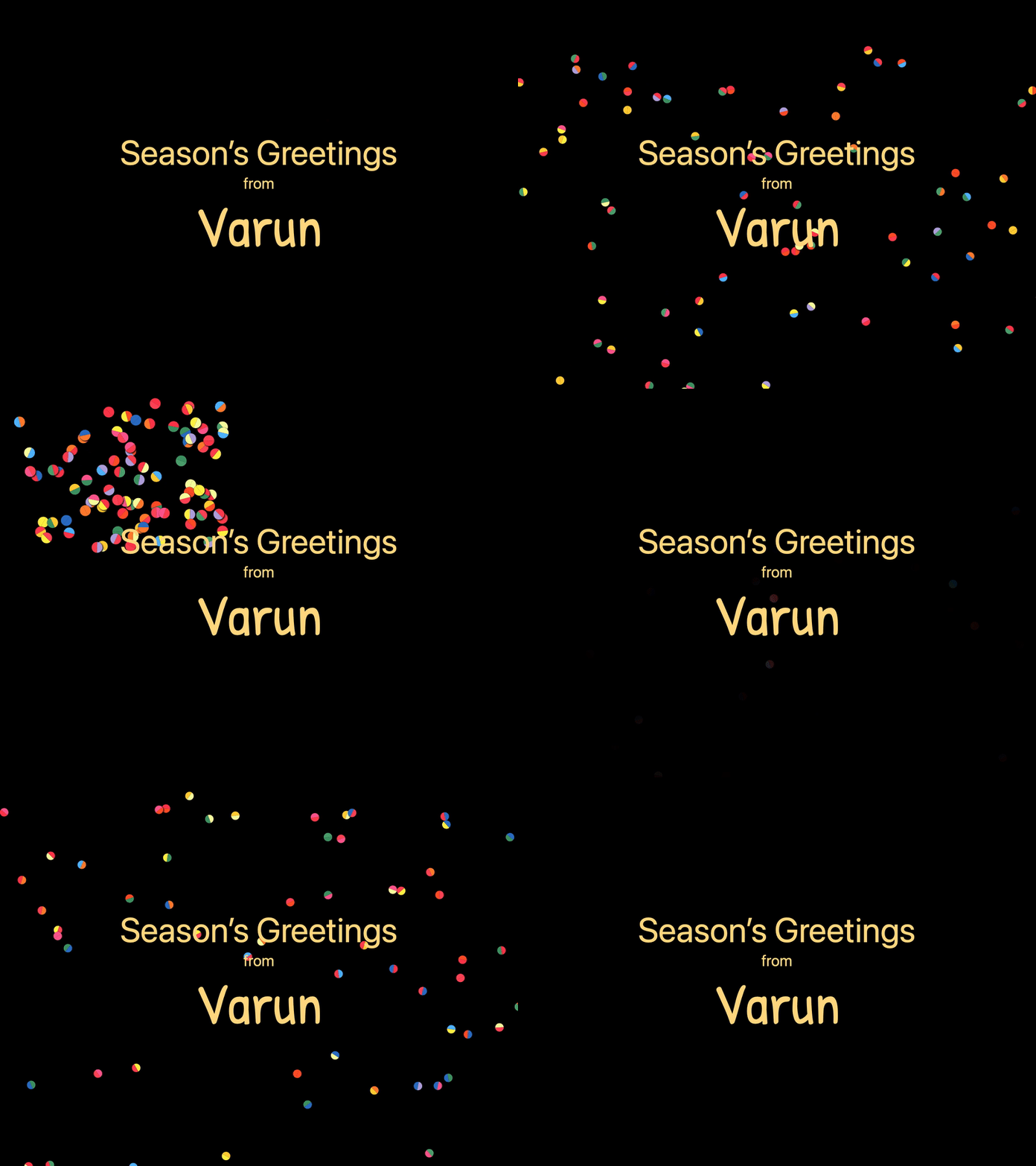
Speaking of particles, noise shows up in particle systems too. For effects like rain, snow or confetti, you’re looking to simulate a natural-looking motion. Imagine a confetti particle floating down to earth. The particles don’t move in straight lines. They float and wiggle due to air resistance. Noise is a really great tool for adding in that organic variability.
const wiggle = {
  x: simplex.noise2D(particle.x * frequency, time) * amplitude,
  y: simplex.noise2D(particle.y * frequency, time) * amplitude,
};
particle.x += wiggle.x;
particle.y += wiggle.y;
For a deeper dive, check my post on building a confetti cannon 🎉
Shaders
Let’s circle all the way back to those animated blobs. Manipulating and animating 3D geometries is a lot more efficient with shaders. But shaders are a whole different world unto themselves. For starters, there is a special WebGL version of noise, glsl-noise. We’ll need to import that into our shader using glslify.
We’ll take it slow, starting with 2D first.
The animation above is quite similar to the contours we looked at earlier. It’s implemented as a fragment shader. Which means we run the same program for each pixel of the canvas.
Notice the pragma line? That’s us importing webgl-noise. Then use it to generate noise data for each pixel position vUv.
This part should look quite familiar by now.
precision highp float;
uniform float time;
uniform float density;
varying vec2 vUv;

#define PI 3.141592653589793
#pragma glslify: noise = require(glsl-noise/simplex/3d);

float patternZebra(float v){
  float d = 1.0 / density;
  float s = -cos(v / d * PI * 2.);
  return smoothstep(.0, .1 * d, .1 * s / fwidth(s));
}

void main() {
  // Generate noise data  float amplitude = 1.0;  float frequency = 1.5;  float noiseValue = noise(vec3(vUv * frequency, time)) * amplitude;  // Convert noise data to rings
  float t = patternZebra(noiseValue);
  vec3 color = mix(vec3(1.,0.4,0.369), vec3(0.824,0.318,0.369), t);
  // Clip the rings to a circle
  float dist = length(vUv - vec2(0.5, 0.5));
  float alpha = smoothstep(0.250, 0.2482, dist);

  gl_FragColor = vec4(color, alpha);
}
Fragment shaders have this concept of distance functions used for drawing shapes. patternZebra is one such example that converts noise data into rings. Essentially it returns either 0 or 1. Which we then use to pick a colour using mix. And finally, use another distance function to clip a circular boundary.
Seems quite basic?
Well, the amazing thing about shaders is that you can turn them into a material and apply it to more complex geometry.
Noise Material
We can take the same 2D mars shader from above. Convert it into a ThreeJS shader material. Then use the vertex position vPosition to generate noise instead of vUv.
And voilà, we have a 3D Mars!
const material = new THREE.ShaderMaterial({
  extensions: {
    derivatives: true,
  },
  uniforms: {
    time: { value: 0 },
    density: { value: 1.0 },
  },
  vertexShader: /*glsl*/ `
    varying vec3 vPosition;
    void main () {
      vPosition = position;
      gl_Position = projectionMatrix * modelViewMatrix * vec4(position, 1.0);
    }
    `,
  fragmentShader: glslify(/* glsl */ `
    precision highp float;
    varying vec3 vPosition;
    uniform float time;
    uniform float density;
    #pragma glslify: noise = require(glsl-noise/simplex/4d);
    #define PI 3.141592653589793
    float patternZebra(float v){
      float d = 1.0 / density;
      float s = -cos(v / d * PI * 2.);
      return smoothstep(.0, .1 * d, .1 * s / fwidth(s));
    }
    void main () {
      float frequency = .6;
      float amplitude = 1.5;
      float v = noise(vec4(vPosition * frequency, sin(PI * time))) * amplitude;
      float t = patternZebra(v);
      vec3 fragColor = mix(vec3(1.,0.4,0.369), vec3(0.824,0.318,0.369), t);
      gl_FragColor = vec4(fragColor, 1.);
    }
    `),
});This is honestly just a start. Shaders open up so many possibilities. Like the example below 👻
Not only is noise mapping to colours but, also alpha.
Glossy Blobs
The idea behind vertex displacement is quite similar. Instead of a fragment shader, we write a vertex shader that transforms each vertex of the sphere. Again, applied using a shader material.
precision highp float;
varying vec3 vNormal;

#pragma glslify: snoise4 = require(glsl-noise/simplex/4d)

uniform float u_time;
uniform float u_amplitude;
uniform float u_frequency;

void main () {
  vNormal = normalMatrix * normalize(normal);  float distortion = snoise4(vec4(normal * u_frequency, u_time)) * u_amplitude;  vec3 newPosition = position + (normal * distortion);
  gl_Position = projectionMatrix * modelViewMatrix * vec4(newPosition, 1.0);
}
Oh, and throw on some matcap, and you’ve got some glossy animated blobs.
Your turn to make some noise
That was quite a journey. Motion, textures, fields, particle systems and displacement—noise can do it all. It truly is the workhorse of the creative coding world.
So obviously, you want to play with noise 😁
I’ve put together a little starter CodePen for you. It spins up a grid of noise and maps it to an array of glyphs. Just start by modifying the array and see how far you can take it.
const glyphs = ['¤', '✳', '●', '◔', '○', '◕', '◐', '◑', '◒'];Or if you’re looking for something more advanced, check out noisedeck.app. It’s like a synthesizer but for visuals.
Either way, don’t forget to share your creations with me on Twitter.
